How does a 3D model reach the browser?
Loading a file in Three.js is the visible result. The more useful questions are what the file describes, what the browser needs, and which approximations connect the two.
First, what does this “model” describe?
A radio and an industrial part can both rotate on screen while using very different representations. The radio may combine triangle meshes, textures and materials; a cylindrical CAD face can instead be described by a surface definition, boundaries and adjacency. Similar images can come from different data structures.
I separate source representation from display representation. Digital content creation tools (DCC), such as Blender and C4D, typically organize assets around appearance. Industrial CAD commonly uses boundary representation (B-rep) for precise geometry. B-rep includes not only surfaces but the boundaries of each face and the relationships that close a solid. Appearance and geometric precision are different priorities, not absolute divisions between tools.
- Meshes + materials + textures
- glTF / GLB
- GLTFLoader → Three.js
- Surfaces and topology in STEP
- OpenCASCADE parsing & tessellation
- In-memory mesh → Three.js / GLB
Figure: two source files converge on mesh rendering. STL and OBJ are possible intermediate formats, but are not required by this implementation.
STEP is an exchange format, not a guarantee that a CAD application’s full parametric history survives. This example uses B-rep STEP. STEP also represents B-spline surfaces, and some protocols support tessellated representations, so “STEP never contains triangles” is not a general rule. We retain the original STEP as the conversion baseline and regenerate derived meshes when needed.
Path one: where does appearance come from?
Start with Microsoft’s public BoomBox asset. GLB is a binary container for glTF, capable of packaging scene descriptions, geometry buffers and images together. The loader assembles scene nodes, reads vertex positions, normals and texture coordinates, and creates mesh materials. The camera determines the view; lighting and materials determine the visible colors.
Orbit with the original material, then switch to solid color. Details that disappear depend on the material or textures; details that still alter the silhouette come from geometry. Wireframe exposes the triangle distribution. Normal mode colors surface orientation, not temperature or stress. Solid and normal modes omit the source normal map, making the underlying geometry easier to inspect.
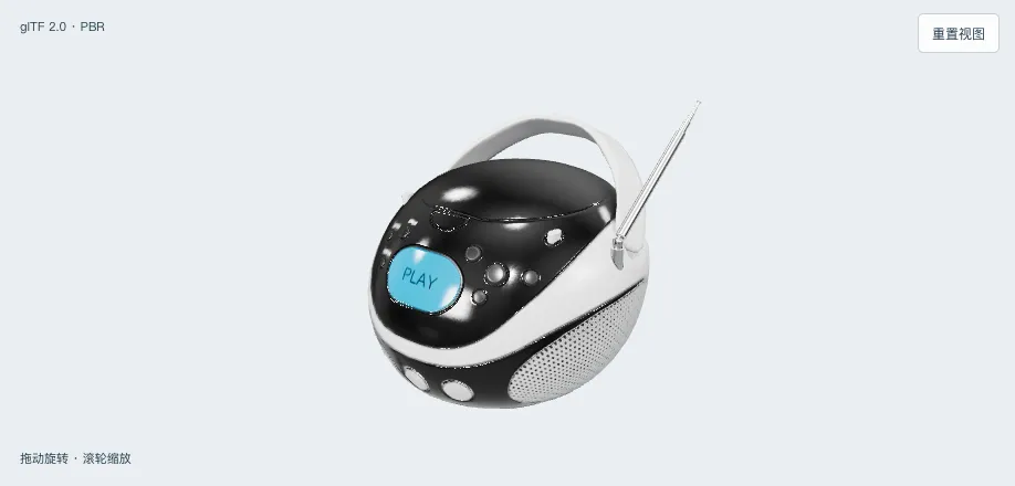 Load the public model · about 10.6 MB
Asset: Microsoft BoomBox, CC0. Lighting uses a procedural room environment and is not the original author’s prescribed setup.
Separate loading from drawing
// Three.js 0.185.1 · 本页实现的核心路径 / core path
const gltf = await loader.parseAsync(glbBytes, "");
scene.add(gltf.scene);
renderer.render(scene, camera);
parseAsync interprets the file as scene objects; render draws those objects from the current camera. Orbiting does not require parsing the GLB again: the controller changes the camera and the next draw reuses the geometry and materials. This distinction determines which work belongs to loading and which work responds to interaction.
I retain the source materials and make diagnostic modes reversible display settings. Wireframe and solid color can then be inspected without modifying the asset, and an export will not accidentally bake in the diagnostic material.
Path two: turn a rounded surface into triangles
This STEP test part was exported from FreeCAD and comes from the rounded-cube tests in occt-import-js. The file contains ADVANCED_BREP_SHAPE_REPRESENTATION, ADVANCED_FACE and surface definitions. These describe solids and boundaries, rather than vertex buffers that Three.js can upload directly to the GPU.
OpenCASCADE interprets these entities and generates a discrete mesh according to tessellation settings. Here the kernel runs as WebAssembly in a browser Worker. The main thread receives positions, normals and indices to create BufferGeometry. Changing settings reprocesses the source file and replaces the mesh while preserving the camera position.
Change linear deflection from 1 mm to 0.01 mm, regenerate, and inspect the rounded edge in wireframe. Compare silhouette and triangle count before looking at time. Status labels follow actual execution stages. Parsing and tessellation occur in one kernel call, so there is no invented face-by-face percentage.
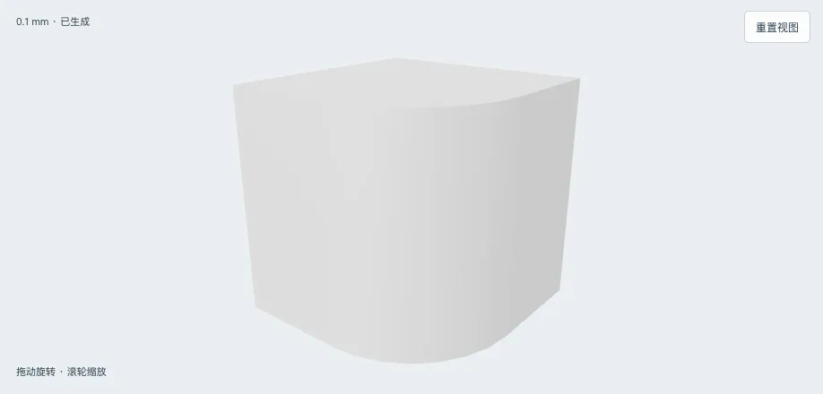 Loads geometry kernel on demand · processed in your browser
// occt-import-js 0.0.23 · Worker 内 / inside the Worker
const result = kernel.ReadStepFile(stepBytes, {
linearUnit: "millimeter",
linearDeflectionType: "absolute_value",
linearDeflection: 0.01,
angularDeflection: 0.5,
});
// positions / normals / indices → BufferGeometryThese settings specify both units and the interpretation of deflection. Here 0.01 means a linear deflection setting of 0.01 mm, not a ratio of the bounding box. Angular deflection stays at 0.5 rad to isolate the linear setting. Both constraints and source geometry tolerances affect the resulting mesh; the parameter is not a measurement of maximum error.
What makes “finer” a useful comparison?
A plane needs few triangles to describe its shape, while curved regions generally require denser sampling. The same setting has different effects on parts of different size and curvature. In this example, both 1 mm and 0.1 mm yield 40 triangles under the fixed angular constraint: tightening one parameter need not immediately change the mesh. Keeping the part, camera and angular deflection fixed helps separate tessellation changes from differences caused by the model or zoom.
The recorded time covers ReadStepFile, including parsing and tessellation, but excludes downloading, WASM startup and drawing. Warm-up can affect the first call, so a finer mesh may be faster in an individual measurement. The table shows observations instead of assuming a monotonic timing curve. Triangle count is not frame rate either: materials, pixel count and the device also affect drawing cost.
The default is a starting point for this particular example. In practice I would select accuracy against visible silhouette, target devices and an explicit cost budget. A smooth appearance does not prove dimensional accuracy, and a display mesh is not the volume mesh required for analysis.
What does a shared GLB format actually unify?
For distribution and repeated viewing, I treat GLB as a display asset. It packages meshes and materials for the browser and can avoid running a CAD kernel on every visit. This STEP experiment processes the source live to expose the approximation. Once the mesh exists, it can be rendered directly without first writing STL, OBJ or GLB.
Choose “Export GLB & verify” in the STEP experiment. The page writes a GLB, reparses it, and checks triangle count and bounds. Kernel output in millimeters is converted to meters. Centering and scaling for the viewport live on a separate parent and are excluded from the export, so making models look equally large on screen does not silently change their delivered dimensions.
This check catches some conversion errors; it cannot recover lost surface precision, CAD feature history or manufacturing semantics. Temperature, stress and flow visualization also need original values and their association with the mesh. VTK’s glTF exporter supports only part of its scene representation. Exporting a contour plot as vertex colors does not transfer the complete scientific dataset.
Keep failures understandable
If the kernel fails to download, the interface does not pretend processing completed. Text and sources remain available without WebGL. Failed regeneration retains the last successful mesh and its settings. Changes that have not been applied are labeled as such, preventing an old image from being mistaken for a new result.
That is my starting point for rendering architecture: source files provide traceability, conversion owns approximation and units, the renderer expresses the result, and the interface makes its identity clear. Those relationships make a visual result useful as engineering evidence.